
This article was originally published in my Digital Tip-A-Month Newsletter. Sign up to get more tips like this in your inbox once a month.
Make your spreadsheets sing with conditional formatting
Even for the most die-hard spreadsheet lover, staring at thousands of rows of numbers will make your eyes glaze over. Charts and graphs are great for helping visualize your aggregate data, but sometimes – especially if you’re a visually-oriented person – you need a way to recognize key bits within the data itself. That’s where conditional formatting can really shine.
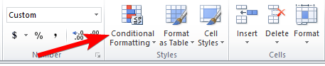
This feature does just what the name says: it lets you automatically apply formatting to cells that meet certain conditions, called rules. To add it, select the cells you want to format, and open up the conditional formatting menu:
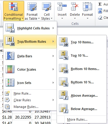
You’ve got a whole range of formatting options:
- Highlight cells in a color if they contain certain text or values – great for calling out blank cells, for instance, which can be hard to see when scanning down a column.
- Highlight the highest or lowest values within a set of cells – great for finding outliers or bright spots within your data.
- Apply icons, bars, or colors to a whole range of cells for a quick visual view of how the values compare to each other.
Let’s look at a few examples:
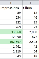
A range of cells with highest values highlighted 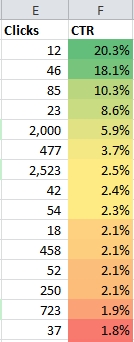
A range of cells color coded by value 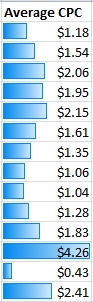
Bars show the relative values of the cells
When I’m analyzing data or assembling a report, I often apply conditional formatting to help me create a narrative in my head for the data. Those colors and icons may not end up in the final report, but they make it easier to identify which points to call out and discuss with my clients.
10-minute Exercise: Learn Conditional Formatting in Excel
Open your nearest spreadsheet – preferably one with long columns of numbers. Select the data in one column, and try applying each type of rule. Play around with the different options, because each one will lend itself to different understandings of your data.
After trying a rule, select the cells again and go to Conditional Formatting > Clear Rules to clear the current formatting before applying a new one. You can also apply multiple rules at once to the same cells!
As you’re working on reporting and analysis, I hope this little trick helps you discover new insights into your data.